This document is part of a series of the analysis of Omics data. Especifically, here is showed how to analyze bulk RNA-Seq data with Bioconductor packages. Also, it’s showcased how to make plots of the RNA data in the context of differentially gene expression and gene-sets.
The analysis of RNA-Seq data involves two distinct parts. The first one needs the use of servers or HPC (high performance computers) and has to do with quality control. pre-processing, alignment-mapping (usually with the STAR software) and counting (can be done using RSEM software). The second one is called downstream analysis and this part involves differential gene expression, gene sets analysis, etc.
Due to the lack of facility to use a server or hpc the first part of the RNA-Seq analysis won’t be done but, you can use the rnaseq pipeline from nfcore. In my experience, the best combination is to use fastq + STAR + RSEM combination of software for this part of the analysis.
With respect to the second part of the analysis, on this document we’ll see how to analyze the airway data set which is a treatment of dexametasome on specific cell lines. Specifically, differentially gene expression, gene sets enrichment analysis and network analysis will be performed.
2 Data & Methods
We are gonna use the airway dataset from the airway package. Part of the analysis will be: - Differential gene expression using DESeq2. - Gene set analysis with fgsea from Cluster profiler. - Network analysis with networkx.
In [1]:
library(airway)
Loading required package: SummarizedExperiment
Warning: package 'SummarizedExperiment' was built under R version 4.3.1
Loading required package: MatrixGenerics
Warning: package 'MatrixGenerics' was built under R version 4.3.1
Loading required package: matrixStats
Warning: package 'matrixStats' was built under R version 4.3.2
The following object is masked from 'package:utils':

    findMatches
The following objects are masked from 'package:base':

    expand.grid, I, unname
Loading required package: IRanges
Attaching package: 'IRanges'
The following object is masked from 'package:grDevices':

    windows
Loading required package: GenomeInfoDb
Warning: package 'GenomeInfoDb' was built under R version 4.3.2
Loading required package: Biobase
Welcome to Bioconductor

    Vignettes contain introductory material; view with
    'browseVignettes()'. To cite Bioconductor, see
    'citation("Biobase")', and for packages 'citation("pkgname")'.
Attaching package: 'Biobase'
The following object is masked from 'package:MatrixGenerics':

    rowMedians
The following objects are masked from 'package:matrixStats':

    anyMissing, rowMedians
library(DESeq2)
Warning: package 'DESeq2' was built under R version 4.3.1
library(tinytex)
Warning: package 'tinytex' was built under R version 4.3.2
library(tidyverse)
Warning: package 'ggplot2' was built under R version 4.3.2
Warning: package 'tidyr' was built under R version 4.3.2
Warning: package 'readr' was built under R version 4.3.2
Warning: package 'purrr' was built under R version 4.3.2
Warning: package 'dplyr' was built under R version 4.3.2
Warning: package 'stringr' was built under R version 4.3.2
Warning: package 'lubridate' was built under R version 4.3.2
Warning: package 'heatmaply' was built under R version 4.3.2
Loading required package: plotly
Warning: package 'plotly' was built under R version 4.3.2
Attaching package: 'plotly'

The following object is masked from 'package:ggplot2':

    last_plot

The following object is masked from 'package:IRanges':

    slice

The following object is masked from 'package:S4Vectors':

    rename

The following object is masked from 'package:stats':

    filter

The following object is masked from 'package:graphics':

    layout

Loading required package: viridis
Warning: package 'viridis' was built under R version 4.3.2
Loading required package: viridisLite

======================
Welcome to heatmaply version 1.5.0

Type citation('heatmaply') for how to cite the package.
Type ?heatmaply for the main documentation.

The github page is: https://github.com/talgalili/heatmaply/
Please submit your suggestions and bug-reports at: https://github.com/talgalili/heatmaply/issues
You may ask questions at stackoverflow, use the r and heatmaply tags:
     https://stackoverflow.com/questions/tagged/heatmaply
======================


Attaching package: 'heatmaply'

The following object is masked from 'package:BiocGenerics':

    normalize
library(htmltools)library(vsn)
Warning: package 'vsn' was built under R version 4.3.1
library(pheatmap)library(genefilter)
Warning: package 'genefilter' was built under R version 4.3.1
Attaching package: 'genefilter'

The following object is masked from 'package:readr':

    spec

The following objects are masked from 'package:MatrixGenerics':

    rowSds, rowVars

The following objects are masked from 'package:matrixStats':

    rowSds, rowVars
library(reticulate)
Warning: package 'reticulate' was built under R version 4.3.2
library(igraph)
Warning: package 'igraph' was built under R version 4.3.2
Attaching package: 'igraph'

The following object is masked from 'package:heatmaply':

    normalize

The following object is masked from 'package:plotly':

    groups

The following objects are masked from 'package:lubridate':

    %--%, union

The following objects are masked from 'package:dplyr':

    as_data_frame, groups, union

The following objects are masked from 'package:purrr':

    compose, simplify

The following object is masked from 'package:tidyr':

    crossing

The following object is masked from 'package:tibble':

    as_data_frame

The following object is masked from 'package:GenomicRanges':

    union

The following object is masked from 'package:IRanges':

    union

The following object is masked from 'package:S4Vectors':

    union

The following objects are masked from 'package:BiocGenerics':

    normalize, path, union

The following objects are masked from 'package:stats':

    decompose, spectrum

The following object is masked from 'package:base':

    union
library(apeglm)
Warning: package 'apeglm' was built under R version 4.3.1
library(munsell)library(org.Hs.eg.db)
Loading required package: AnnotationDbi
Warning: package 'AnnotationDbi' was built under R version 4.3.2
Attaching package: 'AnnotationDbi'

The following object is masked from 'package:plotly':

    select

The following object is masked from 'package:dplyr':

    select
library(rols)
Warning: package 'rols' was built under R version 4.3.2
This is 'rols' version 2.30.2


Attaching package: 'rols'

The following object is masked from 'package:AnnotationDbi':

    Term
library(fgsea)
Warning: package 'fgsea' was built under R version 4.3.1
library(GeneTonic)
Warning: package 'GeneTonic' was built under R version 4.3.1
Warning: package 'htmlwidgets' was built under R version 4.3.2
library(viridis)library(clusterProfiler)
Warning: package 'clusterProfiler' was built under R version 4.3.1
clusterProfiler v4.10.0  For help: https://yulab-smu.top/biomedical-knowledge-mining-book/

If you use clusterProfiler in published research, please cite:
T Wu, E Hu, S Xu, M Chen, P Guo, Z Dai, T Feng, L Zhou, W Tang, L Zhan, X Fu, S Liu, X Bo, and G Yu. clusterProfiler 4.0: A universal enrichment tool for interpreting omics data. The Innovation. 2021, 2(3):100141

Attaching package: 'clusterProfiler'

The following object is masked from 'package:AnnotationDbi':

    select

The following object is masked from 'package:igraph':

    simplify

The following object is masked from 'package:purrr':

    simplify

The following object is masked from 'package:IRanges':

    slice

The following object is masked from 'package:S4Vectors':

    rename

The following object is masked from 'package:stats':

    filter
library(scales)
Warning: package 'scales' was built under R version 4.3.2
Attaching package: 'scales'

The following object is masked from 'package:viridis':

    viridis_pal

The following object is masked from 'package:purrr':

    discard

The following object is masked from 'package:readr':

    col_factor
library(visNetwork)
Warning: package 'visNetwork' was built under R version 4.3.2
library(magrittr)
Attaching package: 'magrittr'

The following object is masked from 'package:purrr':

    set_names

The following object is masked from 'package:tidyr':

    extract

The following object is masked from 'package:GenomicRanges':

    subtract
For all the analysis the Himes et al. (2014) dataset will be used. Also, the Love, Huber, and Anders (2014) package will be used for the differential gene expression step.
We can see how the variance is stabilized with the rlog transformation.
In [5]:
rld <-rlog(dds)hex_df<-data.frame(Means=rowMeans(assay(rld)),Sds=rowSds(assay(rld)))gghex<-hex_df |>ggplot(aes(Means,Sds))+geom_hex(alpha=0.8,bins=40)+guides(fill=guide_colourbar(title ="Counts"))+labs(x="Sorted mean of normalized counts per gene",y="Standard deviation of normalized counts per gene")+theme_minimal()+geom_smooth(aes(Means,Sds),colour="red",linewidth=0.5) + paletteer::scale_fill_paletteer_c("ggthemes::Green-Gold")bslib::card(full_screen = T, bslib::card_title("Stabilized Variance"), plotly::ggplotly(gghex))
`geom_smooth()` using method = 'gam' and formula = 'y ~ s(x, bs = "cs")'
Stabilized Variance
Expand
Also, is important to check if appears some structure in the sample to sample distances plot.
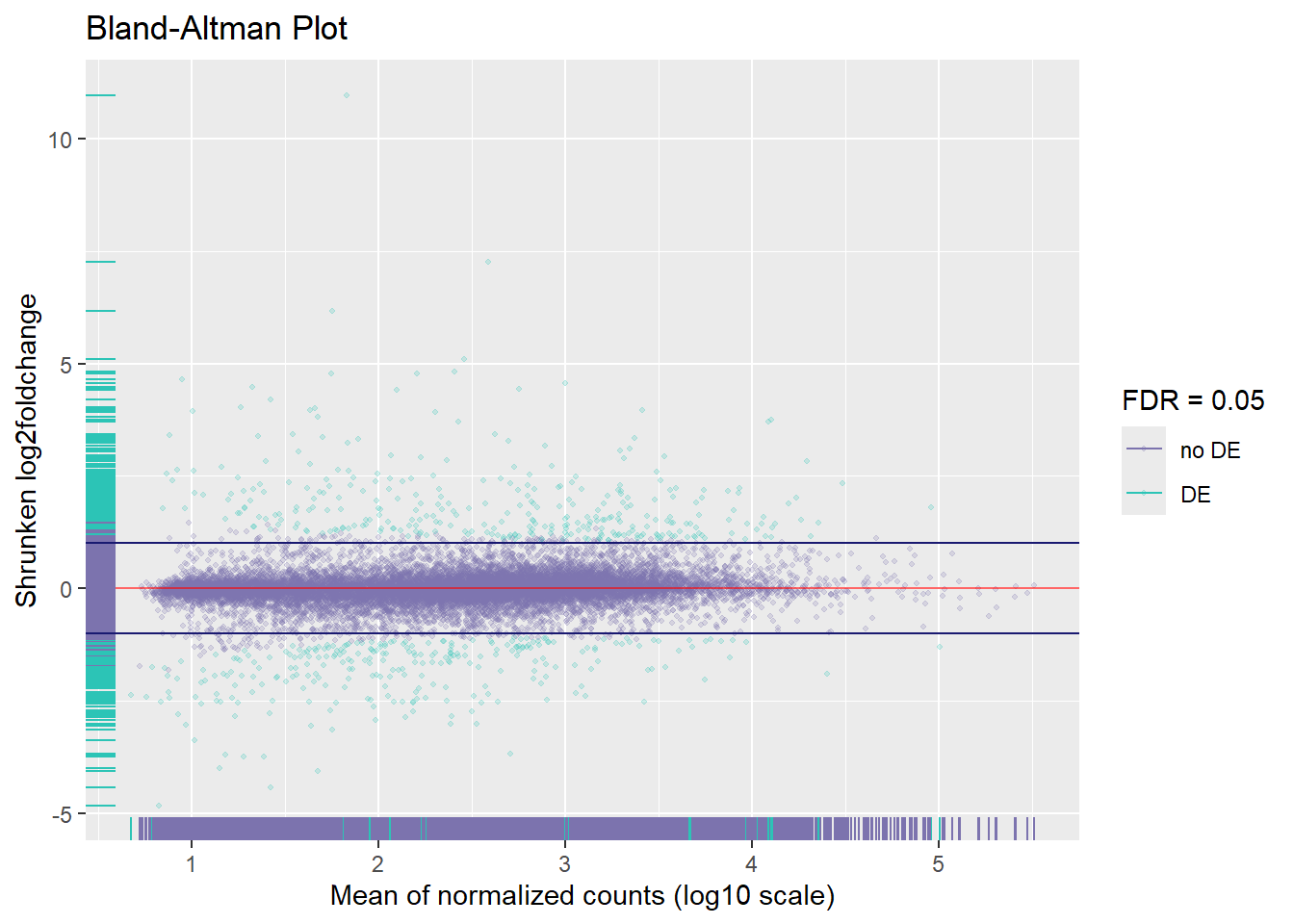
Let’s calculate differential expressed genes using shrinked log2 fold changes with threshold of 1 and a FDR of 0.05.
In [7]:
dds <-DESeq(dds)
using pre-existing size factors
estimating dispersions
gene-wise dispersion estimates
mean-dispersion relationship
final dispersion estimates
fitting model and testing
res <-results(dds, lfcThreshold =1, alpha =0.05, test ="Wald")res.lfc <-lfcShrink(dds, type ="apeglm", lfcThreshold =1, coef =5)
using 'apeglm' for LFC shrinkage. If used in published research, please cite:
    Zhu, A., Ibrahim, J.G., Love, M.I. (2018) Heavy-tailed prior distributions for
    sequence count data: removing the noise and preserving large differences.
    Bioinformatics. https://doi.org/10.1093/bioinformatics/bty895
computing FSOS 'false sign or small' s-values (T=1)
We can see the MA plots as a general view of up and down regulated genes.
As a general view, we can select the top 20 expressed genes ordered by the number of counts.
In [9]:
df<-heatmaply::heatmaply(assay(rld)[select,],col_side_colors=colData(rld)[,c("dex","cell")],colors = viridis::magma(n=256, alpha =0.8, begin =0))bslib::card(df, full_screen = T)
Expand
2.5 Manipulating Annotation with a SQLite DB
For this part of the analysis, is important to use annotation databases, in this case we are gonna use the human h19 genome annotation from the Carlson (2023) package.
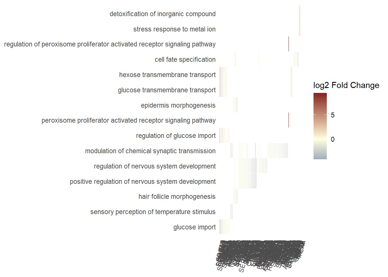
For this part of the process, the Wu et al. (2021) package will be used to make the gene sets enrichment analysis. Is important to mention that for this analysis we are gonna analyze only the biological process ontology,
Warning in preparePathwaysAndStats(pathways, stats, minSize, maxSize, gseaParam, : There are ties in the preranked stats (0.01% of the list).
The order of those tied genes will be arbitrary, which may produce unexpected results.
Using the content of the 'core_enrichment' column to generate the 'gs_genes' for GeneTonic... If you have that information available directly, please adjust the content accordingly.

Using the set of the 'core_enrichment' size to compute the 'gs_de_count'
Found 5414 gene sets in `gseaResult` object, of which 5414 are significant.
---------------------------------
----- GeneTonicList object ------
---------------------------------

----- dds object -----
Providing an expression object (as DESeqDataset) of 16596 features over 8 samples

----- res_de object -----
Providing a DE result object (as DESeqResults), 16596 features tested, 228 found as DE
Upregulated:     142
Downregulated:   86

----- res_enrich object -----
Providing an enrichment result object, 5414 reported

----- annotation_obj object -----
Providing an annotation object of 16596 features with information on 3 identifier types
GeneTonic package have a lot of interactive plots that we can use to dig into our data. An example is a network of Gene sets and genes from which we are gonna perform a network analysis.
In this part of the analysis, we are gonna make a network analysis with Hagberg, Schult, and Swart (2008) networkx library from python. But, before that we need to manipulate the data to have a proper input.
Let’s build a bipartite undirected adjacency matrix.
import pandas as pdimport numpy as npimport networkx as nx
C:\Users\LENOVO\MINICO~1\envs\piero\lib\site-packages\networkx\utils\backends.py:135: RuntimeWarning: networkx backend defined more than once: nx-loopback
  backends.update(_get_backends("networkx.backends"))
import seaborn as sns
from matplotlib import pyplot as plt
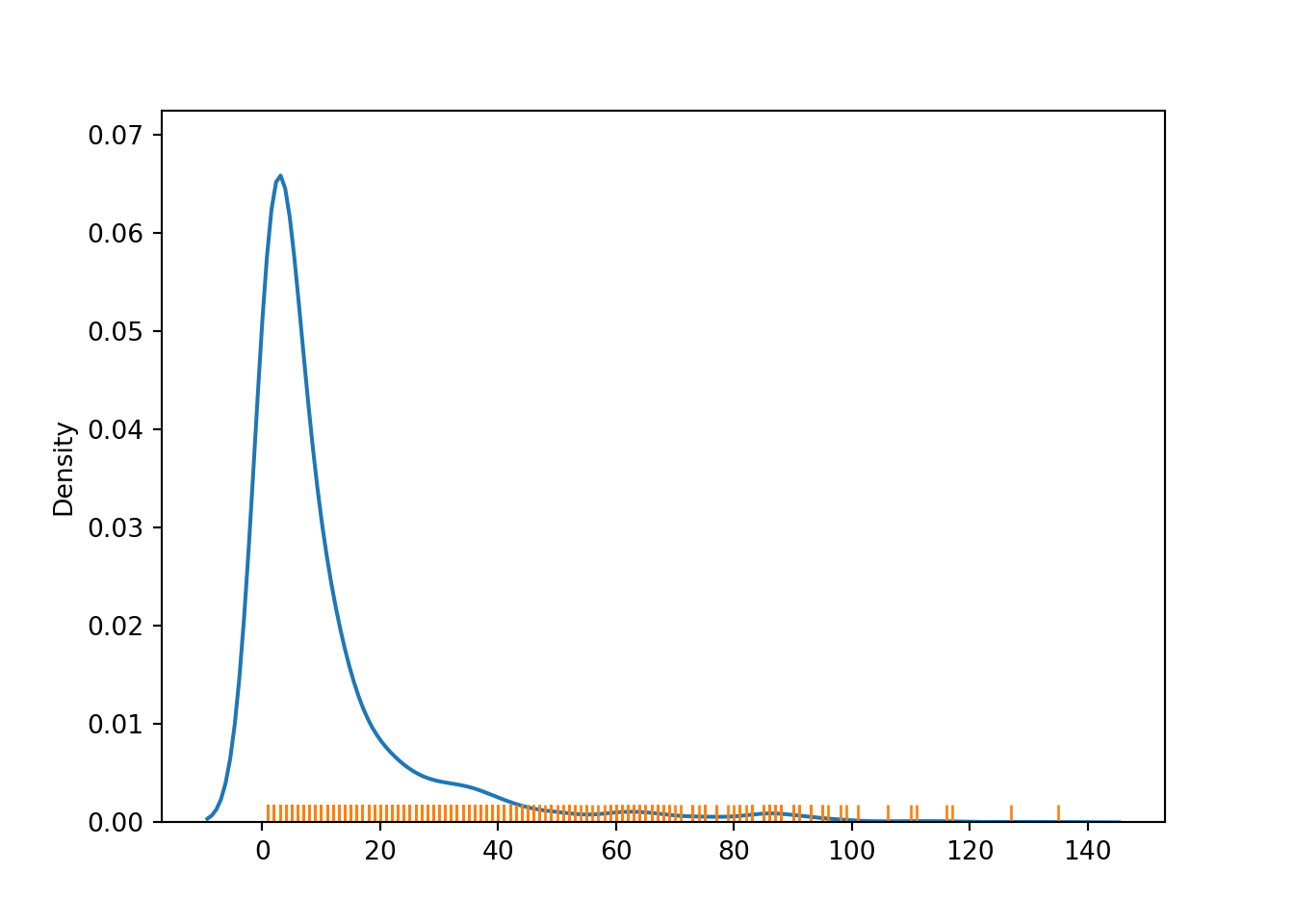
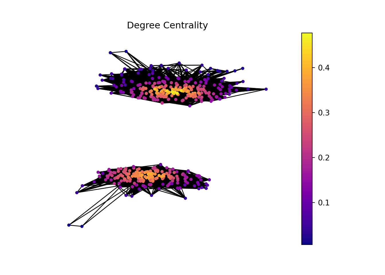
Checking the degree distribution of the graph.
In [17]:
graph = r.adj_matrix_bipartiteG = nx.from_pandas_adjacency(graph, create_using=nx.Graph)degree_sequence =sorted((i[1] for i in G.degree), reverse=True)sns.kdeplot(degree_sequence)sns.rugplot(degree_sequence)plt.show()
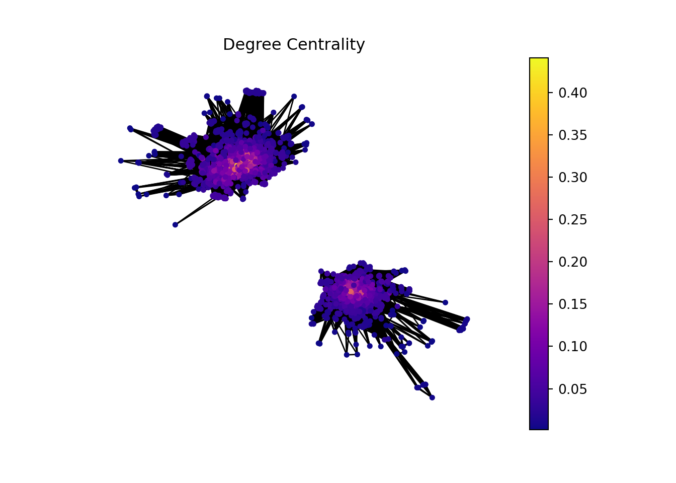
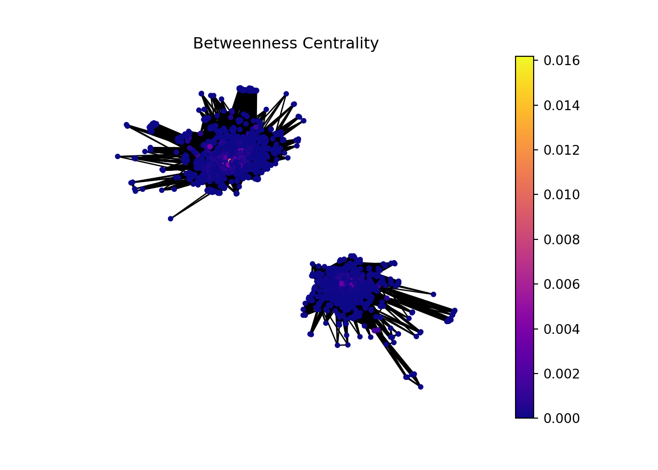
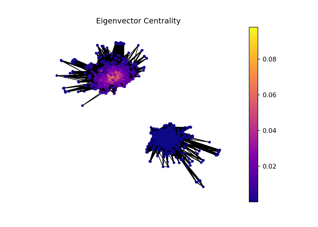
In this plot, we can see that there are two sub graphs with more than 120 connected components. We are gonna work with these.
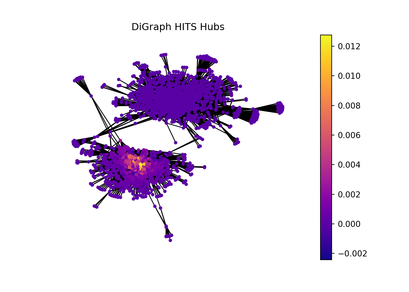
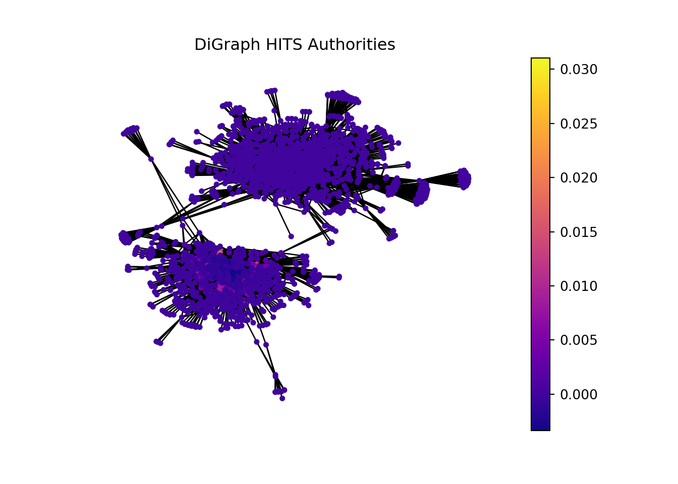
2.8.1 Computing HITS (Hubs and Authorities) Scores.
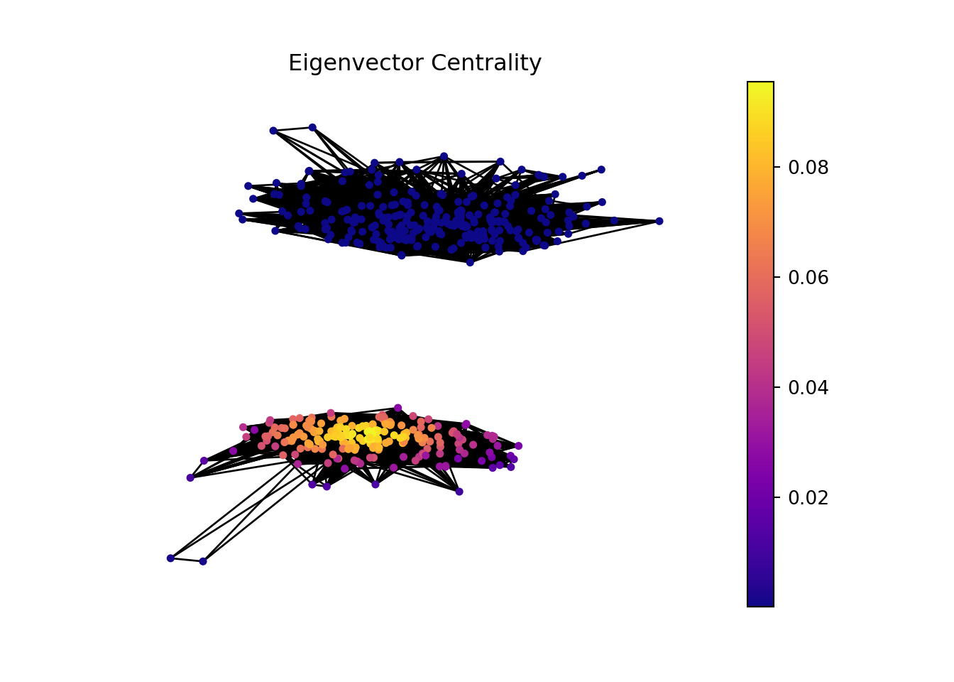
In the context of bioinformatics, applying the concept of hubs and authorities to analyze gene sets and individual genes can offer insightful perspectives on the functional importance and interaction dynamics within genetic networks.
Gene sets or genes with high hub scores may represent critical regulatory functions or be involved in central biological processes. They could be key to understanding disease mechanisms, identifying potential therapeutic targets, or uncovering fundamental aspects of cellular function.
Gene sets or genes identified as high authorities could be central to multiple biological pathways, making them potential biomarkers for diseases or targets for therapeutic intervention. Their importance in various processes makes them subjects of interest for further research and analysis.
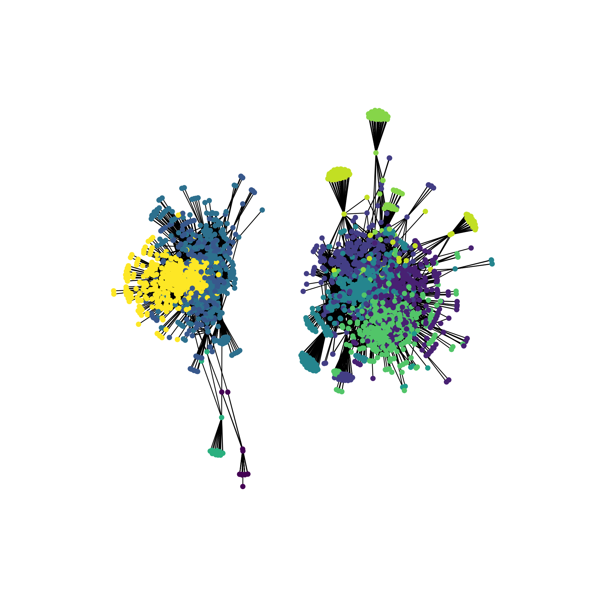
Detecting communities within the network can helps us understand better the underlying biological process.
In [22]:
from community import community_louvainpartitions = community_louvain.best_partition(G)communities = [partitions.get(node) for node in G.nodes()]nx.set_node_attributes(G, partitions, name='community')colors = [G._node[n]['community'] for n in G._node]fig = plt.figure(figsize=(10, 10))ax = fig.add_subplot(111)ax.axis('off')
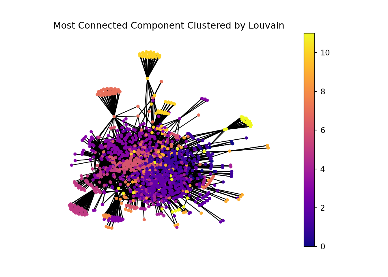
Also, we can focus on the most connected component of the network
In [24]:
components = nx.connected_components(G)largest_component =max(components, key=len)print(f'The largest component have: {len(largest_component)}')
The largest component have: 1580
H = G.subgraph(largest_component)partition = community_louvain.best_partition(H)communities = [partition.get(node) for node in H.nodes()]nx.set_node_attributes(H, partition, name='community')draw(H, spring_pos, partition,'Most Connected Component Clustered by Louvain')
If instead of analysis a bipartite network we want to analyze only gene sets or only genes we need to create two matrices: genesets_coupling matrix and gene_co_expression matrix.
Gene sets similarity can be thought of as the similarity between gene sets based on their shared genes. The strength of the similarity can be measured by the number of genes shared between gene sets.
From a matrix \(G_{mxn}\), with m gene sets and n genes, when can compute the gene set similarity matrix \(S_{mxm}\) (where each element \(s_{ij}\) represents the number of of shared genes between gene sets i and j) as followed:
                                                                                                                                                                                                                            GO:0061687
"Any process that reduces or removes the toxicity of inorganic compounds. These include transport of such compounds away from sensitive areas and to compartments or complexes whose purpose is sequestration of inorganic compounds."
2.10 Gene Co-involvement
Gene co-involvement can be interpreted as the co-involvement of genes in multiple gene sets. The strength of co-involvement can be measured by the number of gene sets in which two genes are both involved.
From a matrix \(G_{mxn}\), with m gene sets and n genes, when can compute the gene set similarity matrix \(C_{mxm}\) (where each element \(c_{ij}\) represents the number of of shared genes between gene sets i and j) as followed:
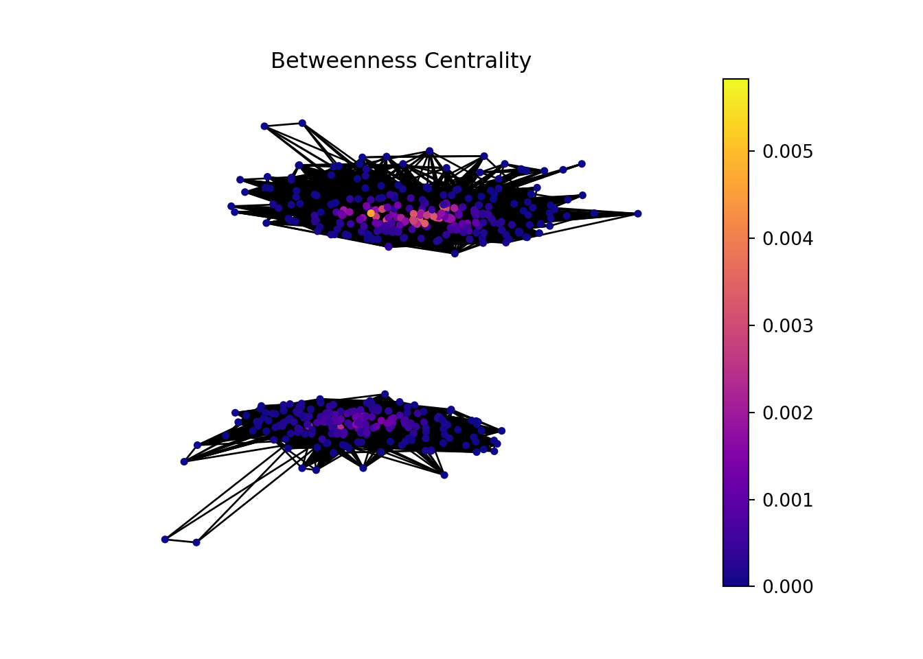
We can sort the table by betweenness centrality to look for genes that serve as bridges or connectors within the network, facilitating the flow of information.
log2 fold change (MLE): dex trt vs untrt
Wald test p-value: dex trt vs untrt
DataFrame with 1 row and 6 columns
                 baseMean log2FoldChange     lfcSE      stat      pvalue
                <numeric>      <numeric> <numeric> <numeric>   <numeric>
ENSG00000174697   116.076        3.02938  0.326588   6.21389 5.16892e-10
                       padj
                  <numeric>
ENSG00000174697 8.66499e-08
3 Conclusion
Differential gene expression analysis was performed on airway dataset.
Gene sets enrichment analysis was performed on airway dataset.
Network analysis was performed on airway dataset.
References
Carlson, Marc. 2023. Org.hs.eg.db: Genome Wide Annotation for Human.
Hagberg, Aric A., Daniel A. Schult, and Pieter J. Swart. 2008. “Exploring Network Structure, Dynamics, and Function Using NetworkX.” In Proceedings of the 7th Python in Science Conference, edited by Gaël Varoquaux, Travis Vaught, and Jarrod Millman, 11–15. Pasadena, CA USA.
Himes, B. E., Jiang, X., Wagner, P., Hu, et al. 2014. “RNA-Seq Transcriptome Profiling Identifies CRISPLD2 as a Glucocorticoid Responsive Gene that Modulates Cytokine Function in Airway Smooth Muscle Cells.”PLoS ONE 9 (6): e99625. http://www.ncbi.nlm.nih.gov/pubmed/24926665.
Love, Michael I., Wolfgang Huber, and Simon Anders. 2014. “Moderated Estimation of Fold Change and Dispersion for RNA-Seq Data with DESeq2” 15: 550. https://doi.org/10.1186/s13059-014-0550-8.
Wu, Tianzhi, Erqiang Hu, Shuangbin Xu, Meijun Chen, Pingfan Guo, Zehan Dai, Tingze Feng, et al. 2021. “clusterProfiler 4.0: A Universal Enrichment Tool for Interpreting Omics Data” 2: 100141. https://doi.org/10.1016/j.xinn.2021.100141.