Code
import numpy as np
import pandas as pd
import matplotlib.pyplot as plt
import scipy as sc
import seaborn as snsimport numpy as np
import pandas as pd
import matplotlib.pyplot as plt
import scipy as sc
import seaborn as snsThe file gamma-ray.csv contains a small quantity of data collected from the Compton Gamma Ray Observatory, a satellite launched by NASA in 1991 (http://cossc.gsfc.nasa.gov/). For each of 100 sequential time intervals of variable lengths (given in seconds), the number of gamma rays originating in a particular area of the sky was recorded.
For this analysis, we would like to check the assumption that the emission rate is constant.
First, let’s check the distribution of the number of gamma rays
df = pd.read_csv("gamma-ray.csv", sep=",")

sns.set_theme(style="darkgrid")
sns.displot(df,x="count")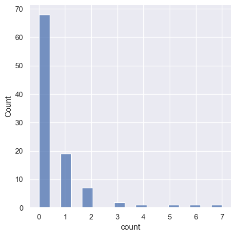
The number of these gamma rays is discrete and non-negative. We can assume that the gamma rays emerge independently of one another, and at constant rate in each time interval. Based on this assumption, a Poisson model is a good model assumption. Each observation \(G_i\) follows a poisson distribution with rate \(\lambda_i\) times the time interval \(t_i\).
\[G_i \thicksim Poisson(\lambda_i * t_i)\]
THe hypothesis that we wanna test is that the emission rate is constat so:
\(H_0: \lambda_0 = \lambda_1 = ... = \lambda_{99}\)
And the alternative hypothesis is that the emisison rates are different:
\(H_A: \lambda_i \neq \lambda_j\) for some i and j
The most plausible parameter for \(\lambda\) under the null hypothesis is the maximun likelihood estimator (MLE).
Given the poisson distribution, the derivation goes as follows:
\[f(G_0,G_1,...,G_{99} | \lambda) = \prod_{i=0}^{99} \frac{e^{-\lambda*t_i}*(\lambda*t_i)^{G_i}}{G_i!}\]
\[ln(f) = -\lambda \sum_{i=0}^{99} t_i + ln(\lambda) \sum_{i=0}^{99} G_i + ln(\prod_{i=0}^{99} t_i^{G_i})) - ln(\prod_{i=0}^{99} G_i!)\]
Then, we derivate w.r.t parameter \(\lambda\) and set the derivative to 0 to find the optimal \(\lambda\).
\[0 = -\sum_{i=0}^{99}t_i + \sum_{i=0}^{99} \frac{G_i}{\lambda}\]
\[\hat{\lambda} = \frac{\sum_{i=0}^{99} G_i}{\sum_{i=0}^{99} t_i}\]
lambda_null = df["count"].sum() / df["seconds"].sum()

lambda_null0.0038808514969907496Similarly, we can calculate a plausible value for the alternative hypothesis with MLE.
\[ln(f) = -\sum_{i=0}^{99} \lambda_i*t_i + \sum_{i=0}^{99} G_i*ln(\lambda_i) + ln(\prod_{i=0}^{99} G_i*ln(t_i)) - ln(\prod_{i=0}^{99} G_i!)\]
WE take the partial derivative w.r.t each parameter \(\lambda_i\) to find the optimal \(\lambda_i\)
\[0 = -t_i + \frac{G_i}{\lambda_i}\]
\[\hat{\lambda_i} = \frac{G_i}{t_i}\]
lambdas_alt = df["count"]/df["seconds"]

lambdas_alt
0 0.000000
1 0.000000
2 0.000000
3 0.000000
4 0.009804
...
95 0.025840
96 0.000000
97 0.000000
98 0.000000
99 0.000000
Length: 100, dtype: float64Now to test these hypotheses, we are gonna use the likelihood ratio test:
\[\Lambda(x) = -2ln(\frac{argmax f(G_0,G_1,...,G_{99}| \lambda)}{argmax f(G_0,G_1,...,G_{99}| \lambda_0,...,\lambda_{99})})\]
which asymptotic distribution \(X_{100-1 = 99}^{2}\)
lh_null = sc.stats.poisson.pmf(k=df["count"], mu=lambda_null)

lh_alt = sc.stats.poisson.pmf(k=df["count"], mu=lambdas_alt)

llh_test = -2*np.log(lh_null.prod() / lh_alt.prod())

llh_test104.33272117042188We can see the distribution of the chi-squared pdf at 99 degrees of freedom
plot_Xs = np.arange(50,150,0.1)
plt.plot(plot_Xs, sc.stats.chi2.pdf(plot_Xs, 99))
plt.show()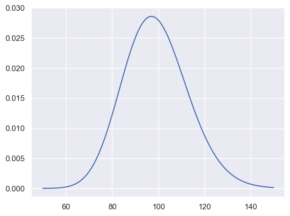
And see the value that give a p-value of 0.05
# We can calculate the Lambda that would give a p-value of 0.05 by using the inverse survival function
sc.stats.chi2.isf(0.05, 99)123.22522145336181Calculating our p-value:
pvalue = sc.stats.chi2.sf(llh_test, 99)
print(pvalue)0.337398546433923We can conclude that we cannot reject our null hypothesis, emission rate of gamma rays appear to be constant.
We are gonna use a dataset from General Motors about mortality. This data is from 59 US cities where it was studied the contribution of air pollution to mortality.
The dependen variable is the age adjusted mortality (Mortality). Also, the data includes variables measuring climate characteristics (JanTemp, JulyTemp, RelHum, Rain), demographic characteristics of the cities (Educ, Dens, NonWhite, WhiteCollar, Pop, House, Income), and variables recording the pollution potential of three diferent air pollutants (HC, NOx, SO2).
Let’s load the data:
df = pd.read_csv("mortality.csv", sep=",")
df.head()| City | Mortality | JanTemp | JulyTemp | RelHum | Rain | Educ | Dens | NonWhite | WhiteCollar | Pop | House | Income | HC | NOx | SO2 | |
|---|---|---|---|---|---|---|---|---|---|---|---|---|---|---|---|---|
| 0 | Akron, OH | 921.87 | 27 | 71 | 59 | 36 | 11.4 | 3243 | 8.8 | 42.6 | 660328 | 3.34 | 29560 | 21 | 15 | 59 |
| 1 | Albany-Schenectady-Troy, NY | 997.87 | 23 | 72 | 57 | 35 | 11.0 | 4281 | 3.5 | 50.7 | 835880 | 3.14 | 31458 | 8 | 10 | 39 |
| 2 | Allentown, Bethlehem,PA-NJ | 962.35 | 29 | 74 | 54 | 44 | 9.8 | 4260 | 0.8 | 39.4 | 635481 | 3.21 | 31856 | 6 | 6 | 33 |
| 3 | Atlanta, GA | 982.29 | 45 | 79 | 56 | 47 | 11.1 | 3125 | 27.1 | 50.2 | 2138231 | 3.41 | 32452 | 18 | 8 | 24 |
| 4 | Baltimore, MD | 1071.29 | 35 | 77 | 55 | 43 | 9.6 | 6441 | 24.4 | 43.7 | 2199531 | 3.44 | 32368 | 43 | 38 | 206 |
Let’s write two helper function that adds the intercept to the data and perform the ordinary least squares estimation based on the formula:
\[\hat{\beta}=(X^{T}X)^{-1}X^{T}y\]
def add_intercept(X: np.array):
  return np.concatenate((np.ones_like(X[:,:1]), X), axis=1)

def OLS(X: np.array, y: np.array):
  return np.linalg.inv(X.T.dot(X)).dot(X.T.dot(y))
Also we need to declare the matrix X and the dependent variable y and convert them to numpy objects.
y = df["Mortality"]
X = df.loc[:,"JanTemp":"SO2"]

# Now lets add the intercept to X

X = X.to_numpy()
y = y.to_numpy()
Now, can calculate the betas:
betas = OLS(add_intercept(X), y)

betas
array([ 1.40003471e+03, -1.44112034e+00, -2.95025005e+00, 1.36009551e-01,
9.69507928e-01, -1.10466624e+01, 4.71706516e-03, 5.30271368e+00,
-1.49231882e+00, 3.40228581e-06, -3.80416445e+01, -4.25186359e-04,
-6.71247478e-01, 1.17850768e+00, 8.45829777e-02])Great! This was an easy way to compute the OLS regression. We also can do the same with sklearn:
from sklearn.linear_model import LinearRegression

reg = LinearRegression()

reg.fit(add_intercept(X),y)

print(reg.intercept_, reg.coef_)
1400.0347123466809 [ 0.00000000e+00 -1.44112034e+00 -2.95025005e+00 1.36009551e-01
9.69507928e-01 -1.10466624e+01 4.71706516e-03 5.30271368e+00
-1.49231882e+00 3.40228581e-06 -3.80416445e+01 -4.25186359e-04
-6.71247478e-01 1.17850768e+00 8.45829777e-02]We also can do the regression task via optimization with the gradient descent algorithm. Let’s write some helper functions that will helps us to do the gradient descent algorithm.
def loss_fn(beta, X, y):
  # (y - X beta)^T (y - X beta)
  return np.sum(np.square(y - X.dot(beta)))

def loss_grad(beta, X, y):
  # -2*(y - X beta)^T X
  return -2*(y - X.dot(beta)).T.dot(X)

def gradient_step(beta, step_size, X, y):
  loss, grads = loss_fn(beta, X, y), loss_grad(beta, X, y)

  beta = beta - step_size * grads.T
  return loss, beta

def gradient_descent(X, y, step_size, precision, max_iter=10000, warn_max_iter=True):
  beta = np.zeros_like(X[0])

  losses = [] # Array for recording the value of the loss over the iterations.
  graceful = False
  for _ in range(max_iter):
    beta_last = beta # Save last values of beta for later stopping criterion
    loss, beta = gradient_step(beta, step_size, X, y)
    losses.append(loss)
    # Use the euclidean norm of the difference between the new beta and the old beta as a stopping criteria
    if np.sqrt(np.sum(np.square((beta - beta_last)))) < precision:
      graceful = True
      break
  if not graceful and warn_max_iter:
    print("Reached max iterations.")
  return beta, np.array(losses)
Before applying the gradient descent, we need to standardize the data because the loss explote due to some outliers. > You can try it without the standardization
# Standardize the data

X_scaled = (X - X.mean(axis=0))/X.std(axis=0, ddof=1)
Y_scaled = (y - y.mean())/y.std(ddof=1)
X_inter = add_intercept(X_scaled)

# Apply the gradient descent

beta_gd, losses = gradient_descent(X_inter, Y_scaled, 0.001, 1e-8, max_iter=10000)
print("BetaHat = {}".format(beta_gd))
print("Final loss value = {}".format(losses[-1]))
plt.plot(range(len(losses)), losses)
plt.title("Iteration vs Loss")
plt.show()

# As a sanity check, we can also do the matrix inversion with OLS
print("Matrix inverse BetaHat = {}".format(OLS(X_inter, Y_scaled)))
Reached max iterations.
BetaHat = [ 9.99200722e-19 -2.34387032e-01 -2.17491727e-01  1.17191047e-02
  1.79800652e-01 -1.50530629e-01  1.08943031e-01  7.64357603e-01
 -1.21223518e-01  8.40179286e-02 -1.11464155e-01 -3.04603568e-02
 -9.95161696e-01  8.80002697e-01  8.62630571e-02]
Final loss value = 13.809259921735789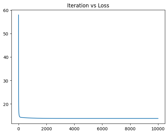
Matrix inverse BetaHat = [ 3.21984155e-17 -2.34377091e-01 -2.17496828e-01  1.17238925e-02
  1.79754504e-01 -1.50544513e-01  1.08945825e-01  7.64348559e-01
 -1.21202349e-01  8.40325965e-02 -1.11479218e-01 -3.04687337e-02
 -9.96190618e-01  8.81043305e-01  8.61146149e-02]
Note that the betas changed because we standardized the data, thats why at the end we are checking with the OLS function.