Integrative Analysis of Multi-omic Data

1 Introduction

2 GWAS Catalog with a ChIP-Seq Experiment

Here, we are gonna analyze the relation between transcription factor binding (ESRRA binding data) from a ChIP-Seq experiment and the genome-wide associations between DNA variants and phenotypes like diseases. For this task, we are gonna use a the gwascat package distributed by the EMBL (European Molecular Biology Laboratories).

In [1]:

library(tidyverse)

Warning: package 'ggplot2' was built under R version 4.3.2

Warning: package 'tidyr' was built under R version 4.3.2

Warning: package 'readr' was built under R version 4.3.2

Warning: package 'purrr' was built under R version 4.3.2

Warning: package 'dplyr' was built under R version 4.3.2

Warning: package 'stringr' was built under R version 4.3.2

Warning: package 'lubridate' was built under R version 4.3.2

── Attaching core tidyverse packages ──────────────────────── tidyverse 2.0.0 ──
✔ dplyr     1.1.4     ✔ readr     2.1.5
✔ forcats   1.0.0     ✔ stringr   1.5.1
✔ ggplot2   3.5.0     ✔ tibble    3.2.1
✔ lubridate 1.9.3     ✔ tidyr     1.3.1
✔ purrr     1.0.2     
── Conflicts ────────────────────────────────────────── tidyverse_conflicts() ──
✖ dplyr::filter() masks stats::filter()
✖ dplyr::lag()    masks stats::lag()
ℹ Use the conflicted package (<http://conflicted.r-lib.org/>) to force all conflicts to become errors

library(gwascat)

Warning: package 'gwascat' was built under R version 4.3.1

gwascat loaded.  Use makeCurrentGwascat() to extract current image.
 from EBI.  The data folder of this package has some legacy extracts.

library(GenomeInfoDb)

Warning: package 'GenomeInfoDb' was built under R version 4.3.2

Loading required package: BiocGenerics

Warning: package 'BiocGenerics' was built under R version 4.3.1

Attaching package: 'BiocGenerics'

The following objects are masked from 'package:lubridate':

    intersect, setdiff, union

The following objects are masked from 'package:dplyr':

    combine, intersect, setdiff, union

The following objects are masked from 'package:stats':

    IQR, mad, sd, var, xtabs

The following objects are masked from 'package:base':

    anyDuplicated, aperm, append, as.data.frame, basename, cbind,
    colnames, dirname, do.call, duplicated, eval, evalq, Filter, Find,
    get, grep, grepl, intersect, is.unsorted, lapply, Map, mapply,
    match, mget, order, paste, pmax, pmax.int, pmin, pmin.int,
    Position, rank, rbind, Reduce, rownames, sapply, setdiff, sort,
    table, tapply, union, unique, unsplit, which.max, which.min

Loading required package: S4Vectors
Loading required package: stats4

Attaching package: 'S4Vectors'

The following objects are masked from 'package:lubridate':

    second, second<-

The following objects are masked from 'package:dplyr':

    first, rename

The following object is masked from 'package:tidyr':

    expand

The following object is masked from 'package:utils':

    findMatches

The following objects are masked from 'package:base':

    expand.grid, I, unname

Loading required package: IRanges

Attaching package: 'IRanges'

The following object is masked from 'package:lubridate':

    %within%

The following objects are masked from 'package:dplyr':

    collapse, desc, slice

The following object is masked from 'package:purrr':

    reduce

The following object is masked from 'package:grDevices':

    windows

library(ERBS)
library(liftOver)

Loading required package: GenomicRanges
Loading required package: rtracklayer

Warning: package 'rtracklayer' was built under R version 4.3.1

Loading required package: Homo.sapiens
Loading required package: AnnotationDbi

Warning: package 'AnnotationDbi' was built under R version 4.3.2

Loading required package: Biobase
Welcome to Bioconductor

    Vignettes contain introductory material; view with
    'browseVignettes()'. To cite Bioconductor, see
    'citation("Biobase")', and for packages 'citation("pkgname")'.


Attaching package: 'AnnotationDbi'

The following object is masked from 'package:dplyr':

    select

Loading required package: OrganismDbi

Warning: package 'OrganismDbi' was built under R version 4.3.1

Loading required package: GenomicFeatures

Warning: package 'GenomicFeatures' was built under R version 4.3.2

Loading required package: GO.db

Loading required package: org.Hs.eg.db

Loading required package: TxDb.Hsapiens.UCSC.hg19.knownGene

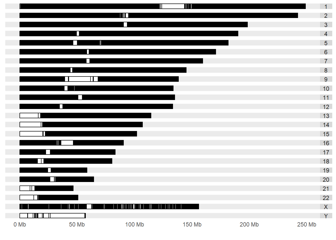
First, we need to download the data, keep the 24 chromosomes (from 1 to Y) and, specify the sequence information from the GRCh38 human genome annotation.

In [2]:

gwcat = get_cached_gwascat()

gg = gwcat |> as_GRanges()

dropping 45505 records that have NA for CHR_POS

1950 records have semicolon in CHR_POS; splitting and using first entry.

3265 records have ' x ' in CHR_POS indicating multiple SNP effects, using first.

gg = keepStandardChromosomes(gg, pruning.mode = "coarse")

# seqlevelsStyle(gg) <- "UCSC"

seqlevels(gg) <- seqlevels(gg) |> 
  sortSeqlevels()

data("si.hs.38")

seqinfo(gg) <- si.hs.38

Now, let’s plot a karyogram that will show the SNP’s identified with significant associations with a phenotype. The SNP’s in the GWAS catalog have a stringent criterion of significance and there has been a replication of the finding from a independent population.

In [3]:

ggbio::autoplot(gg, layout="karyogram")

Registered S3 method overwritten by 'GGally':
  method from   
  +.gg   ggplot2

Scale for x is already present.
Adding another scale for x, which will replace the existing scale.
Scale for x is already present.
Adding another scale for x, which will replace the existing scale.

We can see the peak data as a GRanges object:

In [4]:

data("GM12878")

GM12878

GRanges object with 1873 ranges and 7 metadata columns:
         seqnames            ranges strand |      name     score       col
            <Rle>         <IRanges>  <Rle> | <numeric> <integer> <logical>
     [1]     chrX   1509355-1512462      * |         5         0      <NA>
     [2]     chrX 26801422-26802448      * |         6         0      <NA>
     [3]    chr19 11694102-11695359      * |         1         0      <NA>
     [4]    chr19   4076893-4079276      * |         4         0      <NA>
     [5]     chr3 53288568-53290767      * |         9         0      <NA>
     ...      ...               ...    ... .       ...       ...       ...
  [1869]    chr19 11201120-11203985      * |      8701         0      <NA>
  [1870]    chr19   2234920-2237370      * |       990         0      <NA>
  [1871]     chr1 94311336-94313543      * |      4035         0      <NA>
  [1872]    chr19 45690614-45691210      * |     10688         0      <NA>
  [1873]    chr19   6110100-6111252      * |      2274         0      <NA>
         signalValue    pValue    qValue      peak
           <numeric> <numeric> <numeric> <integer>
     [1]      157.92   310.000        32      1991
     [2]      147.38   310.000        32       387
     [3]       99.71   311.660        32       861
     [4]       84.74   310.000        32      1508
     [5]       78.20   299.505        32      1772
     ...         ...       ...       ...       ...
  [1869]        8.65     7.281   0.26576      2496
  [1870]        8.65    26.258   1.99568      1478
  [1871]        8.65    12.511   1.47237      1848
  [1872]        8.65     6.205   0.00000       298
  [1873]        8.65    17.356   2.01323       496
  -------
  seqinfo: 93 sequences (1 circular) from hg19 genome

If we see the bottom of the GRanges table, this experiment have the hg19 annotation from the human genome. To work on the GRCh38 annotation we need to lift-over with a .chain file. For this we can use the AnnotationHub package.

In [5]:

library(AnnotationHub)

Warning: package 'AnnotationHub' was built under R version 4.3.1

Loading required package: BiocFileCache

Warning: package 'BiocFileCache' was built under R version 4.3.1

Loading required package: dbplyr

Warning: package 'dbplyr' was built under R version 4.3.2

Attaching package: 'dbplyr'

The following objects are masked from 'package:dplyr':

    ident, sql

Attaching package: 'AnnotationHub'

The following object is masked from 'package:Biobase':

    cache

The following object is masked from 'package:rtracklayer':

    hubUrl

ah <- AnnotationHub::AnnotationHub()

query(ah, c("hg19ToHg38.over.chain"))

AnnotationHub with 1 record
# snapshotDate(): 2023-10-23
# names(): AH14150
# $dataprovider: UCSC
# $species: Homo sapiens
# $rdataclass: ChainFile
# $rdatadateadded: 2014-12-15
# $title: hg19ToHg38.over.chain.gz
# $description: UCSC liftOver chain file from hg19 to hg38
# $taxonomyid: 9606
# $genome: hg19
# $sourcetype: Chain
# $sourceurl: http://hgdownload.cse.ucsc.edu/goldenpath/hg19/liftOver/hg19To...
# $sourcesize: NA
# $tags: c("liftOver", "chain", "UCSC", "genome", "homology") 
# retrieve record with 'object[["AH14150"]]' 

chain <- ah[["AH14150"]]

loading from cache

In [6]:

GM12878 <- liftOver(GM12878, chain) |> 
  unlist()

seqlevelsStyle(GM12878) <- "NCBI"

seqinfo(GM12878) <- si.hs.38


seqlevelsStyle(GM12878) <- "UCSC"
seqlevelsStyle(gg) <- "UCSC"

We can find overlaps between the GWAS catalog and the ESRRA ChIP-Seq experiment but, there is a problem; the GWAS catalog is a collection of intervals that reports all significant SNPs and there can be duplications of SNPs associated to multiple phenotypes or the same SNP might be found for the same phenotype in different studies.

We can see the duplications with the reduce function from IRanges package:

In [7]:

# duplicated loci
length(gg) - length(reduce(gg))

[1] 261160

We can see that there are 261160 duplicated loci. Let’s find the overlap between the reduced catalog and the ChIP-Seq experiment:

In [8]:

#
fo = findOverlaps(GM12878, reduce(gg))
fo

Hits object with 613 hits and 0 metadata columns:
        queryHits subjectHits
        <integer>   <integer>
    [1]         6      237757
    [2]         9      221130
    [3]        12       25060
    [4]        15      104699
    [5]        15      104700
    ...       ...         ...
  [609]      1928      246305
  [610]      1929      244698
  [611]      1929      244699
  [612]      1931      250380
  [613]      1931      250381
  -------
  queryLength: 1932 / subjectLength: 268560

We can see 613 hits. Then, we are gonna eobtain the ranges from those hits, retrieve the phenotypes (DISEASE/TRAIT) and show the top 20 most common phenotypes with association to SNPs that lies on the ESRRA binding peaks.

In [9]:

over_ranges <- reduce(gg)[subjectHits(fo)]


ii <- over_ranges |> 
  as.data.frame() |> 
  GenomicRanges::makeGRangesListFromDataFrame()


phset = lapply(ii, function(x){
  
  # print(glue::glue("On range: {x}"))
  unique(gg[which(gg %over% x)]$"DISEASE/TRAIT")
  
})

gwas_on_peaks <- phset |> 
    enframe() |> 
    unnest(value) |> 
    dplyr::count(value) |> 
    slice_max(n, n=20)


p <- gwas_on_peaks |> 
  mutate(value = fct_reorder(value,n)) |> 
  ggplot(aes(n,value, fill=value))+
  geom_col() +
  theme(legend.position = "none") +
  paletteer::scale_fill_paletteer_d("khroma::smoothrainbow") +
  theme_minimal()

htmltools::tagList(list(plotly::ggplotly(p)))

Distinct phenotypes identified on the peaks:

In [10]:

length(phset)

[1] 613

Now, how to do the inference of these phenotype on peaks of these b cells? We can use permutation on the genomic positions to test if the number of phenotypes found is due to chance or not.

In [11]:

library(ph525x)

Loading required package: png

Loading required package: grid

Loading required package: VariantAnnotation

Warning: package 'VariantAnnotation' was built under R version 4.3.2

Loading required package: MatrixGenerics

Warning: package 'MatrixGenerics' was built under R version 4.3.1

Loading required package: matrixStats

Warning: package 'matrixStats' was built under R version 4.3.2

Attaching package: 'matrixStats'

The following objects are masked from 'package:Biobase':

    anyMissing, rowMedians

The following object is masked from 'package:dplyr':

    count

Attaching package: 'MatrixGenerics'

The following objects are masked from 'package:matrixStats':

    colAlls, colAnyNAs, colAnys, colAvgsPerRowSet, colCollapse,
    colCounts, colCummaxs, colCummins, colCumprods, colCumsums,
    colDiffs, colIQRDiffs, colIQRs, colLogSumExps, colMadDiffs,
    colMads, colMaxs, colMeans2, colMedians, colMins, colOrderStats,
    colProds, colQuantiles, colRanges, colRanks, colSdDiffs, colSds,
    colSums2, colTabulates, colVarDiffs, colVars, colWeightedMads,
    colWeightedMeans, colWeightedMedians, colWeightedSds,
    colWeightedVars, rowAlls, rowAnyNAs, rowAnys, rowAvgsPerColSet,
    rowCollapse, rowCounts, rowCummaxs, rowCummins, rowCumprods,
    rowCumsums, rowDiffs, rowIQRDiffs, rowIQRs, rowLogSumExps,
    rowMadDiffs, rowMads, rowMaxs, rowMeans2, rowMedians, rowMins,
    rowOrderStats, rowProds, rowQuantiles, rowRanges, rowRanks,
    rowSdDiffs, rowSds, rowSums2, rowTabulates, rowVarDiffs, rowVars,
    rowWeightedMads, rowWeightedMeans, rowWeightedMedians,
    rowWeightedSds, rowWeightedVars

The following object is masked from 'package:Biobase':

    rowMedians

Loading required package: SummarizedExperiment

Warning: package 'SummarizedExperiment' was built under R version 4.3.1

Loading required package: Rsamtools

Warning: package 'Rsamtools' was built under R version 4.3.1

Loading required package: Biostrings

Warning: package 'Biostrings' was built under R version 4.3.2

Loading required package: XVector

Warning: package 'XVector' was built under R version 4.3.1

Attaching package: 'XVector'

The following object is masked from 'package:purrr':

    compact

Attaching package: 'Biostrings'

The following object is masked from 'package:grid':

    pattern

The following object is masked from 'package:base':

    strsplit

Attaching package: 'VariantAnnotation'

The following object is masked from 'package:stringr':

    fixed

The following object is masked from 'package:base':

    tabulate

library(progress)

Warning: package 'progress' was built under R version 4.3.3

set.seed(123)

n_iter = 100

pb <- progress_bar$new(format = "(:spin) [:bar] :percent [Elapsed time: :elapsedfull || Estimated time remaining: :eta]",
                       total = n_iter,
                       complete = "=",   # Completion bar character
                       incomplete = " ", # Incomplete bar character
                       current = ">",    # Current bar character
                       clear = FALSE,    # If TRUE, clears the bar when finish
                       width = 100)   


rsc = sapply(1:n_iter, function(x) {
    pb$tick()
    length(findOverlaps(reposition(GM12878), reduce(gg))) |> 
    suppressWarnings()
    
})

# compute prop with more overlaps than in observed data
mean(rsc > length(fo))

[1] 0

3 Explore the TCGA

Please check the dedicated script (top left) to see how to explore and get insights from the TCGA (The Cancer Genome Atlas) database.

4 Conclusion

References